Building a parking space detector with Computer Vision [Part 1]

Creating the Machine Learning model. Publicado originalmente en The Deep Hub.

Car park which we will be analyzing | Source

This project is the beginning of a series featured by The Deep Hub in which we will be creating end-to-end Machine Learning projects. Check it out here.

Analyzing the problem
Masking fundamentals
Segmenting the image with a mask
Training a Convolutional Neural Network
Integrating the model with OpenCV

The idea of parking slot detectors is not something new. I´m sure that you´ve seen at least one time a car park with a counter keeping track of the amount of available free slots in it.

Traditional methods have been primarily based on manual systems which consisted of placing mobility sensors in each parking lot to detect occupancy.

This solution is effective but very expensive and maintenance-intensive; Imagine having to install 1000 mobility sensors, one for each parking space…

How we can improve this with Machine Learning?

With computer vision, the approach would be to place one camera (or more if needed) in a strategic place where all the parts in the car park could be recorded.

The camera would be able to detect the slots that are occupied with a Machine Learning model. A much more efficient solution, since we would just have to install the camera(s), instead of placing for example 200 mobility sensors.

Parking slot detector | Source

Analyzing the problem

As in every other machine-learning case, the first thing we should ask ourselves is if we really need a machine-learning approach to solve the problem.

In this case, we have various options. Let´s go through all of them.

Object detection model

One popular approach would be to use an object detection model such as YOLO (You Only Look Once) or R-CNN (Region-based Convolutional Neural Networks) which we could train to predict the location of the slots and classify whether they are empty or occupied.

Example of an object detection model | Source

What do we need to train an object detection model?

To train one of these neural networks we need a very big amount of data comprised of images annotated with their locations and classification.

(e.g., in the figure above the algorithm is predicting the dimensions of the object and the class it belongs to).

Normally these special datasets are stored in YOLO, COCO (Common Objects in Context), or Pascal VOC (Visual Object Classes) formats which store the labeling of object classes and their spatial locations within an image.

Preparing for this task involves several steps:

Data Collection: Amass a diverse set of parking lot images under various conditions (e.g., different times of day, and weather conditions).
Annotation: Label the images with accurate bounding boxes around each parking slot and categorize each as ‘occupied’ or ‘empty’.
Dataset Preparation: Organize the annotated data in a structured format like YOLO, COCO, or Pascal VOC.

Bounding box format: COCO vs YOLO Bounding box format: COCO vs YOLO | Source

An object detection model may not be the best option…

The approach of training an object detection model is alright, however in this case it might not be the best thing to do.

Think about it, YOLO normally is used when we have to predict the position of an object, but in this case, we don´t have to.

The parking slots are always in the same place!

This means we have half of the work done, we just need to classify each of the parking spaces in whether they are occupied or not.

Training an object detection model is hard because you have to create an annotated dataset including the coordinates and category of each object.This is useful when we have to predict the position in which an object will be or its dimensions. However in this case it doesn´t make much sense as the parking lots are always in the same place and always have the same dimensions.

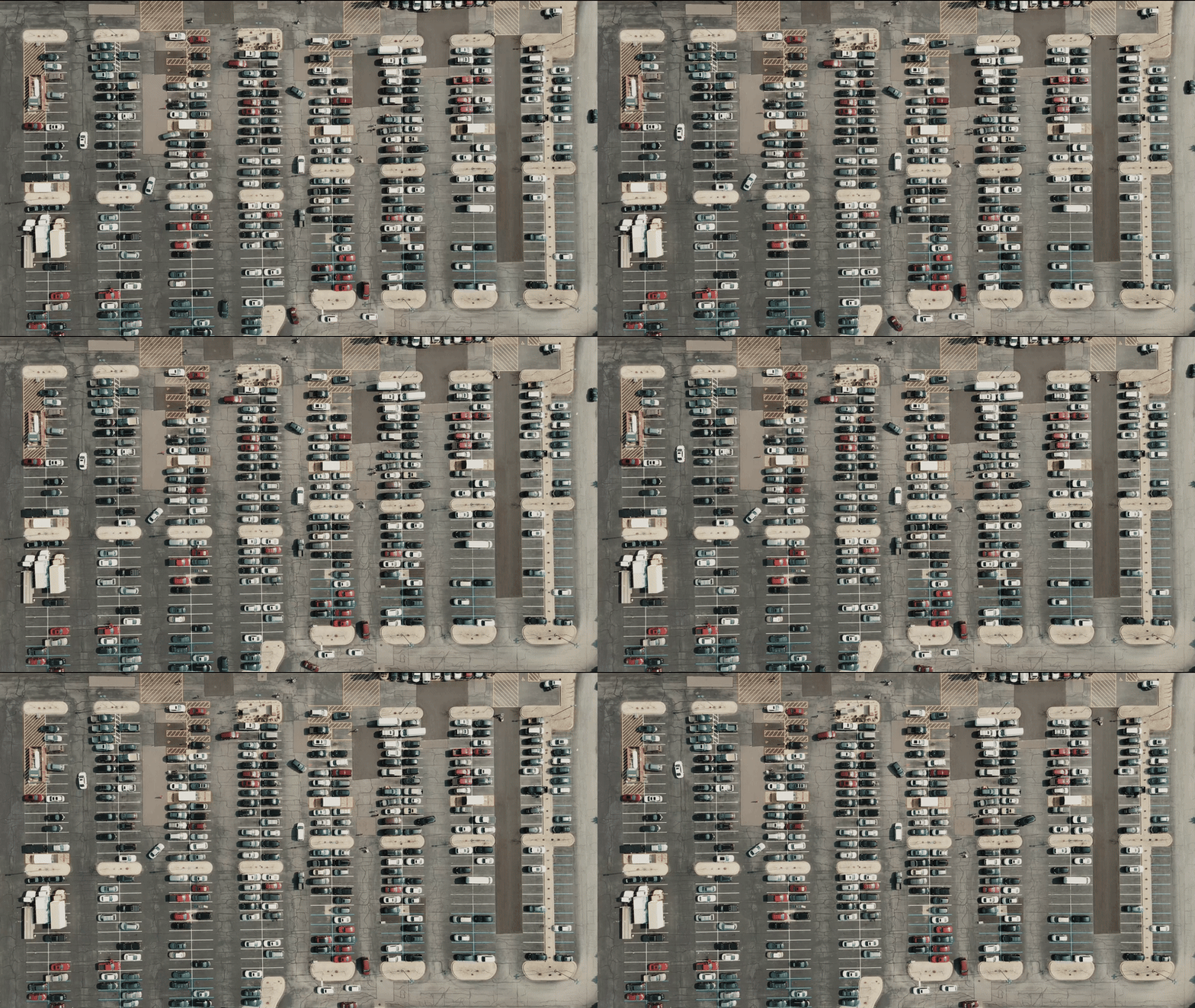The camera doesn´t move, the parking slots are always in the same place | Source

Great! But even if we know where the slots will be located. How can we pass their respective location and dimensions to a model that will classify them as occupied or not?

Here comes the first part of the project. Building a mask!

Masking fundamentals

Masking is a technique used to isolate specific portions of images or videos so that operations can be performed on those areas alone.

It’s like giving the computer a way to focus on particular objects while ignoring the rest.

Binary vs RGB mask Binary vs RGB mask | Source

In this figure, a mask is created to isolate the giraffe in the picture with Binary and RGB masks.

In our case, the model won´t need information about the colors to identify whether the parking slots are occupied or not so we will create a binary mask.

Building the mask

To build the mask we have various options. Perhaps the most popular and automatic one is the OpenCV library.

However in this case we want to create a more customized mask that covers each of the slots in the car park. We could try to do this with OpenCV, however, it might be too complex so I will build it manually.

Some popular tools with which you can create a mask are:

(If you´d like to recommend any other you can leave a suggestion in the comments).

For the sake of simplicity and not extending too much this explanation I picked a mask from the YouTube channel Computer vision engineer who built a customized one for this specific video file using Inkscape.

You can check out how he created the mask in his Patreon.

Original image and mask | Source

As you can see in the above figures, the mask highlights only the parking slots and doesn´t take into account the rest.

The approach will be to select each of these slots and pass them to our model which will classify whether they are occupied or not.

Let´s see how we can combine our mask with the original video file.

Segmenting the image with the mask

As you will see in a moment, this is a very simple operation and OpenCV will make it even easier for us.

Let´s go through some coding!

You´ll have to import the mask and the original video. You can download them here.

If you are not familiar with OpenCV you can check out their documentation. Anyways we won´t be creating a very complex program so you might be able to follow it without any problem.

import cv2

mask_image_path = r"path\to\your\mask"
video_path = r"path\to\your\video"

video_capture = cv2.VideoCapture(video_path)
mask = cv2.imread(mask_image_path, cv2.IMREAD_GRAYSCALE)

Awesome! Now that we have loaded the files let´s see how we can join them together.

Before we dive in, let’s clarify one thing about video files:

A video is essentialy a compilation of numerous images linked in sequence*.* These individual images are known as frames.- When working with a video, we engage in processing a loop of frames*,* applying transformations to each of these “linked images” within the loop.

Here is a code snippet of how you might load a video with OpenCV.

while video_capture.isOpened():
    ret, frame = video_capture.read()

    if not ret:
       print("Failed to read frame from video or end of video reached.")
       break

    # Display the frame
    cv2.imshow('Processed Video', processed_frame)

    # Break the loop if 'q' is pressed
    if cv2.waitKey(1) & 0xFF == ord('q'):
        break

# Release the video capture object and close all windows
video_capture.release()
cv2.destroyAllWindows()

Inside the loop, video_capture.read() is called to read the next frame from the video source. This method returns two values:

ret: A boolean value indicating whether the frame was successfully read. It’s True if the frame has been successfully grabbed and can be decoded/returned, and False if no frames are available (e.g., if the end of the video has been reached).
frame: The actual frame read from the video. It’s a matrix of pixels if ret is True, or None if ret is False.

The last “if” condition enables you to break the loop if necessary by pressing the q’ key.

Awesome, now that we understand better how video files work let´s go through the steps we need to follow to combine the mask with our video.

# Step 1: Converting each frame into grayscale.

gray = cv2.cvtColor(frame,cv2.COLOR_BGR2GRAY)

This line converts the input frame from BGR (Blue, Green, Red) color space to grayscale using OpenCV’s cvtColor function.

Grayscale conversion is done to simplify the operation since color information is not necessary and working with just one channel will be easier.

# Step 2: Applying the mask

segmented = cv2.bitwise_and(gray, gray, mask=mask)

The cv2.bitwise_and function performs a bitwise AND operation between the gray image and itself, using mask as the mask.

This operation zeroes out all the pixels in gray that are not defined in mask, segmenting the image.

The bitwise operation compares each bit of the first operand to the corresponding bit of the second operand. If both bits are 1, the result bit is set to 1; otherwise, it’s set to 0.

Binary mask representation Binary mask representation | Source

# Step 3: Applying an algorithm to find the contours in the image.

contours,_=cv2.findContours(segmented,cv2.RETR_EXTERNAL,cv2.CHAIN_APPROX_SIMPLE)

The function retrieves only the external contours (cv2.RETR_EXTERNAL) and compresses horizontal, vertical, and diagonal segments into their endpoints only.

How contours are detected in binary images | Source

# Step 4: Draw bounding boxes

Once we have performed these three steps we know the exact location of each parking slot and we can create a square around them with a little bit of Opencv manipulation.

for contour in contours:
    x, y, w, h = cv2.boundingRect(contour)
    cv2.rectangle(frame, (x, y), (x+w, y+h), (0, 255, 0), 2)
return frame

x, y, w, h = cv2.boundingRect(contour): For each contour, this line computes the smallest rectangle that can enclose it by calling cv2.boundingRect(contour). The function returns four values:

x and y: The coordinates of the top-left corner of the bounding rectangle.
w and h: The width and height of the bounding rectangle, respectively.

cv2.rectangle(frame, (x, y), (x+w, y+h), (0, 255, 0), 2): This line draws a rectangle on the frame using the rectangle’s top-left corner (x, y) and the bottom-right corner (x+w, y+h).

The rectangle is drawn with the following properties:

(0, 255, 0): The color of the rectangle, specified in BGR (Blue, Green, Red) format. It is set to green with full intensity (255) and no blue or red.
2: The thickness of the lines that make up the rectangle.

Great, now that we´ve gone through all the steps, let´s define our function:

def draw_bounding_boxes(frame, mask):
    gray = cv2.cvtColor(frame, cv2.COLOR_BGR2GRAY)
    segmented = cv2.bitwise_and(gray, gray, mask=mask)
    contours, _ = cv2.findContours(segmented, cv2.RETR_EXTERNAL, 
                                              cv2.CHAIN_APPROX_SIMPLE)
    for contour in contours:
        x, y, w, h = cv2.boundingRect(contour)
        cv2.rectangle(frame, (x, y), (x+w, y+h), (0, 255, 0), 2)
    return frame

Easy enough right?

Now we will update the code to include this function in our loop.

This is what we have for now in our main program:

Main script to combine our mask with the original video file | Código en https://github.com/TheDeepHub/ParkingDetector

If you installed the necessary dependencies and added the correct paths to your downloaded video and mask you should see something like this:

Mask combined with the video file | Created by the author

Awesome!

Once we have created the mask the process is quite straightforward.

Let´s go through the next steps.

But do we really need to train a machine-learning model?

In computer vision, the solution to our problems is not always CNNs!

You should always analyze the case, and evaluate if we need a neural network to solve it.

Changes in pixel intensity

If you pay attention, the parking slots always have the same color intensity. This simplifies in a great measure the process.

The problem could be solved in the following way:

Parking slots always have the same pixel intensity, if this changes then it means that a car has occupied it.

Car leaving a parking slot and changing the pixel intensity | Source

We can detect a change in pixel intensity with a histogram of gradients (among many other methods). Easy pixel manipulation.

This solution seems perfect as it is very fast and efficient, however, it´s not so robust.

What if a pedestrian walks into the parking slot?
What if is a rainy or foggy day, the pixel intensity might also change.
What if the camera is not cleaned?

All these external situations make this approach a bit weak.

By analyzing better all these conditions, we could create a system able to adapt to all these changes in the pixel intensity.

However, for the sake of simplicity (and because probably is what you are looking for) we will train a CNN!

Training a Convolutional Neural Network with TensorFlow

If you´re reading this post, I suppose you have some idea about CNNs, if you don´t you can take a look at my article for the theoretical concepts you need to know!

Convolutional Neural Networks: A Comprehensive Guide Exploring the power of CNNs in image analysis

To classify the parking slots depending on whether they are occupied or not we will train a CNN classifier. This is a good approach since we have a great dataset and the neural network will be simple to train.

We will use Python and TensorFlow, a very popular framework for Machine Learning.

In the first place, we have to import the dataset. Normally what is done with images is to store each category in a different folder.

Images stored in two different directories | Created by the author

In this case, we only have two classes:

empty
not_empty

Each category contains 3.045 images.

Importing an image dataset with TensorFlow

If you´re new to this field you might be more familiar with importing tabular data (which is usually more straightforward with libraries such as pandas).

With images, the process is not so simple. However, TensorFlow makes it very easy for us. There are various ways in which we can create the dataset.

I will use the flow_from_directory()method.

You will have to store the images in directories for this to work.

import tensorflow
from tensorflow.keras.preprocessing.image import ImageDataGenerator

data_gen = ImageDataGenerator(
    rescale=1./255,
    validation_split=0.2)

dataset_path = "/path/to/dataset"
train_ds = data_gen.flow_from_directory(
    directory=dataset_path,
    subset="training",
    seed=123,
    target_size=(29,68),
    batch_size=32,
    class_mode='sparse',
    shuffle=True)

val_ds = data_gen.flow_from_directory(
    directory=dataset_path,
    subset="validation",
    seed=123,
    target_size=(29, 68),
    batch_size=32,
    class_mode='sparse',
    shuffle=True)

Let´s review what is happening here:

In the first place, we are creating an ImageDataGenerator instance. Here we define the transformations we will apply to the dataset. In this case, I will only rescale them and define the percentage of the dataset that will be included in the validation set.

Rescaling is normally done for several reasons, primarily to normalize the data and make the model training process more efficient and stable.

Tensorflow pipeline with ImageDataGenerator Tensorflow pipeline with ImageDataGenerator | Source

Once we have defined all the transformations we want to apply to the dataset we start with flow_from_directory().

Let´s review some of the most important parameters of this method.

directory: Path to the target directory containing subdirectories, each of which should contain images belonging to one class.
subset: Subset in which the dataset will be split (train, val, or test).
target_size: The dimensions to which all images will be resized. (29, 68) is selected because is the average dimension in the dataset.
batch_size: Number of images to be yielded from the generator per batch.

The images are resized via interpolation, there are three main methods used in OpenCV: bilinear, bicubic, and nearest neighbors interpolation.

The Art and Science of Interpolation Exploring the pillars of image processing

To know more about this function check out the documentation in TensorFlow.

Building the model

Awesome now that we imported the dataset, let´s build the model.

In the field of computer vision, it is common to use pre-built convolutional neural networks rather than building models from scratch.

On this occasion, since the task is very simple and we just have to classify two outcomes, I will build the architecture from scratch by myself.

I will include:

2 Convolutional layers
2 max-pooling layers
1 flattened layer
2 dense layers

You can visualize it in the figure below.

Structure of the CNN Structure of the CNN | Source: Created by the author with visualkeras library

To build this architecture we have various options. I will use the Sequential API.

The Sequential API is a great starting point for building neural networks in TensorFlow due to its simplicity and ease of use.

import tensorflow as tf
from tensorflow.keras.models import Sequential
from tensorflow.keras.layers import Conv2D, MaxPooling2D, 
                                    Flatten, Dense, Dropout

# Model architecture
model = Sequential([
    Conv2D(32, (3, 3), activation='relu', input_shape=(29, 68, 3)),
    MaxPooling2D(2, 2),
    Conv2D(64, (3, 3), activation='relu'),
    MaxPooling2D(2, 2),
    Flatten(),
    Dense(128, activation='relu'),
    Dropout(0.5),
    Dense(2, activation='softmax')])

If you want to know more about how the Sequential API works and about other ways of creating a neural network architectures, check out this article:

Sequential vs Functional vs Subclassing API in Tensorflow Choosing the best architecture for your model

Compiling the model

The compilation is an essential step in building and training a neural network.

This phase prepares the model for training by specifying key properties such as the loss function, optimizer, and metrics to monitor.

I will use the Adam optimizer and the accuracy metric.

The loss will be the sparse_categorical_crossentropy which works with integer labels.

It is called “sparse” because you don’t need to convert your class labels into a dense one-hot encoded array; you can simply use the direct integer labels.

model.compile(optimizer='adam',
              loss='sparse_categorical_crossentropy',
              metrics=['accuracy'])

Training the model

In the training phase, the model learns to make predictions by adjusting its weights based on the input data and the specified loss function.

This process involves feeding the training data into the model, comparing the model’s predictions against the actual outcomes, and then updating the model’s weights to minimize the loss.

To indicate the number of times this process will be done, we create a determined number of epochs.

epochs = 10
history = model.fit(
    train_ds,
    validation_data=val_ds,
    epochs=epochs)

In this gist you can see how the complete script will look:

CNN training script | Código en CNN_Model/Train_CNN.ipynb

If you´ve uploaded the training dataset correctly the program should work for you.

In the following figure, you can see the results we obtained:

Convolutional Neural Network results | Created by the author

It´s important to analyze this correctly.

The first accuracy indicates the results in the training dataset and the “val_accuracy” is the result obtained from the validation dataset.

We always have to check the second “accuracy” score to prevent overfitting.

Theory apart, the results were great, with just 10 epochs we were able to obtain a 99.1% accuracy.

This means our model should perform all right in almost all the cases.

In order to mimick the whole process of training a neural network we included a hyper parameter tuning section in the repository. I won´t go through it in this tutorial but you can check it out here!

Saving the weights

Once created the model we just have to save the weights. In this way, we´ll be able to load the model from an external program and incorporate it into our program.

model.save('/content/model/path_to_model.H5')

The model is usually saved in a .H5 file. This file is saved in the Hierarchical Data Format (HDF5).

HDF5 is a high-performance data format designed to store and organize large amounts of data making it versatile for different scientific fields and applications.

If you want to know more about it check out this article:

The HDF5 File The purpose of this chapter is to describe how to work with HDF5 data files. If HDF5 data is to be written to or read…

Integrating the model with our program

Now that we have built the model, we must include it in our program.

To do this the process is quite straightforward.

In the first place, we´ll have to create a preprocessing function to adapt the frames that we analyze to our model’s first layer which was designed to accept images with a size of (68, 29).

Once we have done this we will normalize it.

We´ll also have to include another dimension as our model will be processing the images into batches.

This will be our preprocessing function:

def preprocess_for_prediction(roi, target_size=(68, 29)):
    # Resize the ROI to the target size expected by the model
    roi_resized = cv2.resize(roi, target_size)
    # Normalize pixel values if your model expects normalization
    roi_normalized = roi_resized / 255.0
    # Expand dimensions to add the batch size
    roi_expanded = np.expand_dims(roi_normalized, axis=0)
    return roi_expanded

Now we have to integrate the model with our program. Remember the main script we built for segmenting the video with a mask?

We´ll just have to modify it a bit to integrate it with our neural network.

Take a look at the new function:

def draw_bounding_boxes_and_predict(frame, mask, model):
    gray = cv2.cvtColor(frame, cv2.COLOR_BGR2GRAY)
    segmented = cv2.bitwise_and(gray, gray, mask=mask)
    contours, _ = cv2.findContours(segmented, cv2.RETR_EXTERNAL, cv2.CHAIN_APPROX_SIMPLE)

    for contour in contours:
        x, y, w, h = cv2.boundingRect(contour)
        # Extract ROI using the bounding box coordinates
        roi = frame[y:y+h, x:x+w]
        # Preprocess the ROI for model prediction
        roi_preprocessed = preprocess_for_prediction(roi)
        # Predict the occupancy using your model
        prediction = model.predict(roi_preprocessed)
        predicted_class = np.argmax(prediction, axis=1)[0]  # Assuming binary classification: 0 for empty, 1 for occupied
        
        # Draw bounding box in green if empty, red if occupied
        color = (0, 255, 0) if predicted_class == 0 else (0, 0, 255)
        cv2.rectangle(frame, (x, y), (x+w, y+h), color, 2)

    return frame

In essence, we are performing the same operations as before, but now we are including a preprocessing step, a prediction step, and a new condition to make the bounding box red if our model predicted that the parking slot is occupied or green if not.

Awesome, now we have it all set up for our main program. We´ll be using only two functions:

preprocess_for_prediction()
draw_bounding_boxes_and_predict()

This will be our main script:

Main script | Código en main.py

Only 20 lines of code!?

Yep, we don´t need much more. If you followed all the steps correctly you should have something similar to the following output:

Final result | Created by the author

A review of what we´ve done so far:

We created a mask to isolate the parking spaces.
We trained a convolutional neural network to classify between occupied and not-occupied.
We integrated our model within a loop to detect in each frame the amount of slots available in the car park.

It wasn´t that hard, right? With just a few lines of code, we were able to create a parking slot classifier.

However, we didn´t finish! This is an end-to-end project… Remember?

Now we have to put our model into production.

In part 2 we will see how to deploy and host a Machine Learning model!

A hint: We´ll use Azure and Docker!

Bibliography

Do you have any idea for improving the model or are you building something similar? Let us know in the comments!

Would you like to contribute to this section? Check out this guide.

Make sure to follow us to stay updated with our content!

The Deep Hub Your data science hub. A Medium publication dedicated to exchanging ideas and empowering your knowledge.