The Art and Science of Interpolation

Exploring the pillars of image processing. Publicado originalmente en The Deep Hub.

Photo by Jakob Owens on Unsplash

Image interpolation is a computational process used in digital image processing to estimate unknown pixel values. It comes into play when images are resized, or transformed, or when missing parts need to be filled in.

The essence of interpolation lies in creating a smooth transition between known pixel values, thereby generating new pixels in a way that maintains the overall integrity and quality of the image.

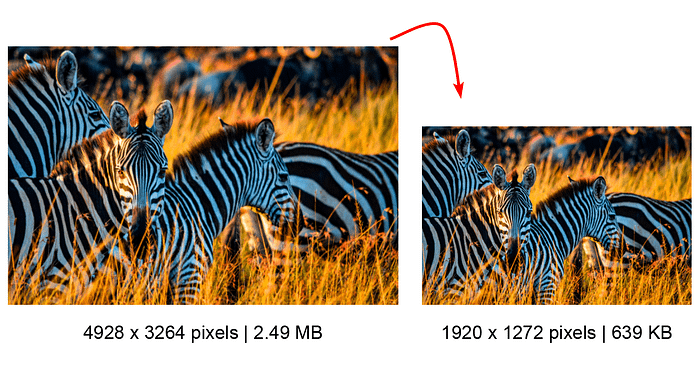Resizing an image | Source

If you are not familiar with pixels and images take a look at the following article:

But how are images created? A quick introduction to pixels and color channels.

How interpolation works

At a fundamental level, image interpolation methods rely on surrounding known pixel values to calculate the unknown or new pixel values.

This can be visualized as filling in the blanks in a grid of pixels, where the “blanks” are the new pixels that need to be created.

The goal is to make these new pixels blend seamlessly with the existing ones, preserving edges, textures, and gradients as accurately as possible.

Resizing

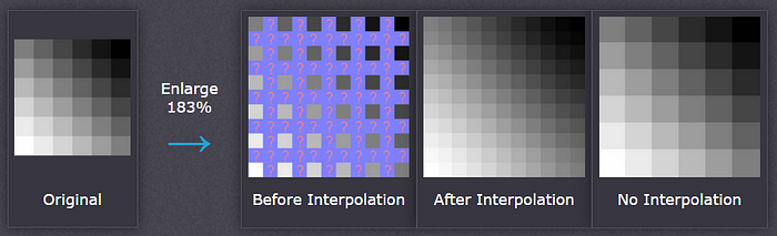Image resizing with interpolation | Source

In the figure above we can see more clearly the process of interpolation. With the actual pixels, we have to estimate the new pixels that will be added to the image once we enlarge or downsample it.

Rotating

Image rotation with interpolation | Source

Another common example of interpolation is rotating an image. Here we are also applying this technique to rotate the picture into different angles.

The more you know about the surrounding pixels, the better the interpolation will become.Results quickly deteriorate the more you stretch an image, and interpolation can never add detail which is not already present to your picture.

Types of interpolation

1. Nearest neighbor interpolation
2. Bilinear interpolation
3. Bicubic interpolation

# Nearest neighbor interpolation

The simplest form of interpolation. It assigns the value of the nearest pixel to the new pixel.

This method is fast but can result in a blocky, less smooth image.

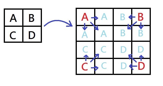Nearest neighbor interpolation upsampling| Source

# Bilinear interpolation

Bilinear interpolation considers the closest 2 × 2 neighborhood of known pixel values surrounding the unknown pixel.

It then takes a weighted average of these 4 pixels to arrive at its final interpolated value. This results in much smoother-looking images than the nearest neighbor.

Bilinear interpolation upsampling | Source

# Bicubic interpolation

Bicubic goes one step beyond bilinear by considering the closest 4 × 4 neighborhood of known pixels — for a total of 16 pixels.

Since these are at various distances from the unknown pixel, closer pixels are given a higher weighting in the calculation.

Bicubic produces noticeably sharper images than the previous two methods and is perhaps the ideal combination of processing time and output quality.

Bicubic interpolation is a standard in many image editing programs (including Adobe Photoshop), printer drivers, and in-camera interpolation.

Example of interpolation

I´ll pick an image from Unsplash and downsample it to see the whole process.

Photo by Silje Midtgård on Unsplash

Before resampling the image, I´ll analyze its dimensions to see the resolution.

You can download the image and keep track of the code of this tutorial.

from PIL import Image
image path = '/mnt/data/horse_medium_interpolation.jpg'image_info = Image.open(image_path)
image_resolution = image_info.size print(image_resolution)

The image resolution is 800 pixels in width by 533 pixels in height.

I will reduce it by a factor of 8 yielding a downsampled size of 100 pixels in width by approximately 66 pixels in height.

Get Jorgecardete’s stories in your inbox

Join Medium for free to get updates from this writer.

Remember me for faster sign in

Image size (800 × 533) → (100 × 66)

1.- Nearest neighbor method

1.1.- Code

from PIL immport Image
import matplotlib.pyplot as plt# Define the downscale factor
downscale_factor = 8  # Downscale the image using the nearest neighbor method
downscaled_image = original_image.resize(
    (original_image.width // downscale_factor, 
     original_image.height // downscale_factor), Image.NEAREST)# Display the result
plt.figure(figsize=(8, 6))
plt.imshow(downsacale_image)
plt.title('Nearest Neighbor Interpolation')
plt.axis('off')
plt.show()

1.2.- Image Representation

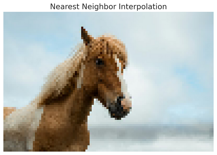Image modified by the author

In the displayed image, you can observe the distinctive visual characteristics nearest neighbor produces:

• Pixelation: The most notable feature is the pixelated appearance, where the individual pixels are enlarged and become visible as distinct squares.
• Jagged Edges: When the image is downscaled and then upscaled, the straight and diagonal lines become jagged, also known as “staircase” due to the abrupt changes in pixel color and intensity.

Use case

This method is computationally less intensive compared to others, making it fast and suitable for real-time applications where processing power is limited.

2.- Bilinear interpolation method

2.1.- Code

from PIL import Image
import matplotlib.pyplot as plt# Define the downscale factor
downscale_factor = 8# Downscale the image using the bilinear method 
downscaled_bilinear = original_image.resize(
    (original_image.width // downscale_factor, 
     original_image.height // downscale_factor), Image.BILINEAR)# Display the downscaled image
plt.figure(figsize=(8, 6))
plt.imshow(downscaled_bilinear)
plt.title('Bilinear Interpolation')
plt.axis('off')
plt.show()

2.2.- Image Representation

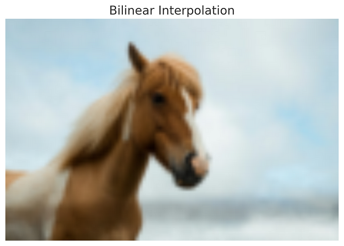Image modified by the author

The bilinear interpolation method represents a significant step up from nearest neighbor interpolation in terms of image quality:

1. Smooth Transitions: Bilinear interpolation calculates the pixel value using a weighted average of the four nearest pixels in the original image, resulting in smoother transitions between pixels. This mitigates the blocky appearance seen in nearest neighbor interpolation.
2. Reduced Jaggedness: The staircasing effect on the edges is less pronounced with bilinear interpolation. It offers a moderate improvement in rendering diagonals and curves, which appear smoother and less jagged.

Use case

Bilinear interpolation is a commonly used method that offers a reasonable trade-off between image quality and computational efficiency,

3.- Bicubic interpolation method

3.1.- Code

# Downscale the image using the bicubic method
downscaled_bicubic = original_image.resize(
    (original_image.width // downscale_factor, 
     original_image.height // downscale_factor), Image.BICUBIC)

# Display the downscaled image
plt.figure(figsize=(8, 6))
plt.imshow(downscaled_bicubic)
plt.title('Bicubic Interpolation')
plt.axis('off')
plt.show()

3.2.- Image Representation

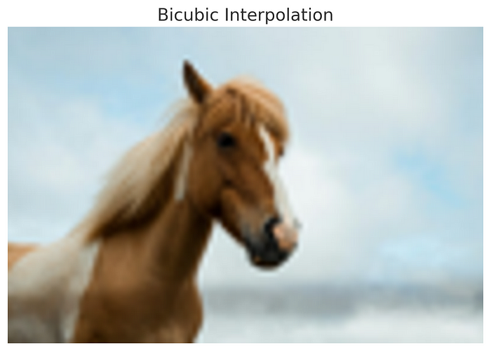Image modified by the author

The bicubic interpolation method is typically used when a high-quality image scaling is required:

1. High-Quality Results: Bicubic interpolation considers the closest 16 pixels (a 4x4 environment) to estimate the new pixel values using cubic polynomials. This results in a higher quality image with smoother edges and finer detail compared to bilinear and nearest neighbor methods.
2. Preservation of Details: It generally does a better job of preserving the details in the image, especially when scaling up. The transitions between different intensities and colors are smoother, which often makes the result look more natural and less digital.

Use case

Bicubic interpolation is the most used technique for resampling images. It is more computationally expensive but usually more effective.

Comparing the different methods

Code

from PIL import Image
import matplotlib.pytplot as pltmethods = {
    "Nearest Neighbor": Image.NEAREST,
    "Bilinear": Image.BILINEAR,
    "Bicubic": Image.BICUBIC
}# Define a larger downscale factor for more pronounced differences
downscale_factor = 8# Downscale and then upscale the image using different interpolation methods
interpolated_images_large_diff = {}
for method_name, method in methods.items():
    # Downscale
    small_image = original_image.resize(
        (original_image.width // downscale_factor, 
         original_image.height // downscale_factor), method)
    # Upscale back to original size
    interpolated_images_large_diff[method_name] = small_image.resize(original_image.size, method)# Display the results
plt.figure(figsize=(15, 10))
plt.subplot(2, 2, 1)
plt.imshow(original_image)
plt.title('Original Image')
plt.axis('off')for i, (method_name, interpolated_image) in enumerate(interpolated_images_large_diff.items(), 2):
    plt.subplot(2, 2, i)
    plt.imshow(interpolated_image)
    plt.title(f'{method_name} Interpolation')
    plt.axis('off')plt.tight_layout()
plt.show()

Image Representation

Overall, each interpolation method has trade-offs between quality and computational complexity.

• The nearest neighbor is the fastest but offers the lowest quality, suitable for real-time applications where speed is critical.
• Bilinear interpolation is a mid-ground, offering a balance between quality and performance.
• Bicubic interpolation provides the highest quality of the three, making it ideal for applications where a high level of detail is necessary.

Bibliography

• https://www.cambridgeincolour.com/tutorials/image-interpolation.htm
• https://www.geeksforgeeks.org/python-opencv-bicubic-interpolation-for-resizing-image/

Thanks for reading! If you like the article make sure to clap (up to 50!) and follow me on Medium to stay updated with my new articles.

Also, make sure to follow my new publication!

The Deep Hub Your data science hub. A Medium publication dedicated to exchanging ideas and empowering your knowledge.